Latent Graph Inference with Limited Supervision

Jianglin Lu^1* Yi Xu¹ Huan Wang¹ Yue Bai¹ Yun Fu^1,2

NeurIPS 2023

¹Department of Electrical and Computer Engineering, Northeastern University
²Khoury College of Computer Science, Northeastern University

^*Corresponding author: jianglinlu@outlook.com

Openreview ArXiv Code

Abstract

Latent graph inference (LGI) aims to jointly learn the underlying graph structure and node representations from data features. However, existing LGI methods commonly suffer from the issue of supervision starvation, where massive edge weights are learned without semantic supervision and do not contribute to the training loss. Consequently, these supervision-starved weights, which may determine the predictions of testing samples, cannot be semantically optimal, resulting in poor generalization. In this paper, we observe that this issue is actually caused by the graph sparsification operation, which severely destroys the important connections established between pivotal nodes and labeled ones. To address this, we propose to restore the corrupted affinities and replenish the missed supervision for better LGI. The key challenge then lies in identifying the critical nodes and recovering the corrupted affinities. We begin by defining the pivotal nodes as k-hop starved nodes, which can be identified based on a given adjacency matrix. Considering the high computational burden, we further present a more efficient alternative inspired by CUR matrix decomposition. Subsequently, we eliminate the starved nodes by reconstructing the destroyed connections. Extensive experiments on representative benchmarks demonstrate that reducing the starved nodes consistently improves the performance of state-of-the-art LGI methods, especially under extremely limited supervision (6.12% improvement on Pubmed with a labeling rate of only 0.3%).

Latent Graph Inference

Existing GNNs typically require a prior graph to learn node representations, which poses a major challenge when encountering incomplete or even missing graphs. This limitation has spurred the development of latent graph inference (LGI), also known as graph structure learning. In general, LGI aims to jointly learn the underlying graph and discriminative node representations solely from the features of nodes. The following gives the definition of latent graph inference.

[Definition 1] (Latent Graph Inference) Given a graph $\mathcal{G}(\mathcal{V}, \mathbf{X} )$ containing $n$ nodes $\mathcal{V}=\{V_1, \ldots, V_n\}$ and a feature matrix $\mathbf{X} \in \mathbb{R}^{n\times d}$ with each row $\mathbf{X}_{i:} \in \mathbb{R}^d$ representing the $d$-dimensional attributes of node $V_i$, latent graph inference (LGI) aims to simultaneously learn the underlying graph topology encoded by an adjacency matrix $\mathbf{A} \in \mathbb{R}^{n\times n}$ and the discriminative $d'$-dimensional node representations $\mathbf{Z} \in \mathbb{R}^{n\times d'}$ based on $\mathbf{X}$, where the learned $\mathbf{A}$ and $\mathbf{Z}$ are jointly optimal for certain downstream tasks $\mathcal{T}$ given a specific loss function $\mathcal{L}$.

In this work, we adopt the most common settings from existing LGI literatures, considering $\mathcal{T}$ as the semi-supervised node classification task and $\mathcal{L}$ as the cross-entropy loss.

Supervision Starvation

Let us consider a general LGI model $\mathcal{M}$ consisting of a latent graph generator $\mathcal{P}_{\mathbf{\Phi}}$ and a node encoder $\mathcal{F}_{\mathbf{\Theta}}$. For simplicity, we ignore the activation function and assume that $\mathcal{F}_{\mathbf{\Theta}}$ is implemented using a $1$-layer GNN, i.e., $\mathcal{F}_{\mathbf{\Theta}}=\mathtt{GNN}_1(\mathbf{X}, \mathbf{A}; \mathbf{\Theta})$, where $\mathbf{A}=\mathcal{P}_{\mathbf{\Phi}}(\mathbf{X})$. For each node $\mathbf{X}_{i:}$, the corresponding node representation $\mathbf{Z}_{i:}$ learned by the model $\mathcal{M}$ can be expressed as: \begin{equation} \mathbf{Z}_{i:} = \mathbf{A}_{i:}\mathbf{X}\mathbf{\Theta} = \left(\sum_{j \in \Omega} \mathbf{A}_{ij}\mathbf{X}_{j:} \right)\mathbf{\Theta}, \end{equation} where $\Omega=\{j\ |\ \mathbb{1}_{\mathbb{R}^+}(\mathbf{A})_{ij}=1 \}$ and $\mathbf{A}_{ij}=\mathcal{P}_{\mathbf{\Phi}}(\mathbf{X}_{i:}, \mathbf{X}_{j:})$. Consider the node classification loss: \begin{equation} \min_{\mathbf{A}, \mathbf{\Theta}} \mathcal{L} = \sum_{i\in \mathcal{Y}_{L}} \sum_{j=1}^{|\mathcal{C}|} \mathbf{Y}_{ij} \ln \mathbf{Z}_{ij} = \sum_{i\in \mathcal{Y}_{L}} \mathbf{Y}_{i:} \ln \mathbf{Z}_{i:}^{\top} = \sum_{i\in \mathcal{Y}_{L}} \mathbf{Y}_{i:} \ln \left( \left(\sum_{j \in \Omega} \mathbf{A}_{ij}\mathbf{X}_{j:} \right)\mathbf{\Theta}\right)^\top, \end{equation} where $\mathcal{Y}_{L}$ represents the set of indexes of labeled nodes and $|\mathcal{C}|$ denotes the size of label set.

We observe that, for $\forall i\in \mathcal{Y}_{L}$, $j \in \Omega$, $\mathbf{A}_{ij}$ is optimized via backpropagation under the supervision of label $\mathbf{Y}_{i:}$. For $\forall i \notin \mathcal{Y}_{L}$, however, if $j \notin \mathcal{Y}_{L}$ for $\forall j \in \Omega$, $\mathbf{A}_{ij}$ will receive no supervision from any label and, as a result, cannot be semantically optimal after training. Consequently, the learning models exhibit poor generalization as the predictions of testing nodes inevitably rely on these supervision-starved weights. This phenomenon is referred to as Supervision Starvation (SS), where many edge weights are learned without any label supervision.

We may ask why this problem arises? In fact, the SS problem is caused by a common and necessary post-processing operation known as graph sparsification, which is employed in the majority of LGI methods to generate a sparse latent graph. To be more specific, graph sparsification adjusts the initial dense graph to a sparse one through the following procedure: \begin{equation} \mathbf{A}_{ij}=\left\{ \begin{aligned} &\mathbf{A}_{ij}, & \text{if } \ \mathbf{A}_{ij} \in \operatorname{top-\kappa}(\mathbf{A}_{i:}) \\ & 0, & \text{otherwise}, \end{aligned} \right. \end{equation} where $\operatorname{top-\kappa}(\mathbf{A}_{i:})$ denotes the set of the top $\kappa$ values in $\mathbf{A}_{i:}$. After this sparsification operation, a significant number of edge weights are directly erased, including the crucial connections established between pivotal nodes and labeled nodes.

How many important nodes or connections suffer from this problem? We delve into this question in the next section.

Starved Nodes

To count how many nodes suffer from the supervision starvation problem, we first give the definition of the k-hop starved node:

[Definition 2] (k-hop Starved Node) Given a graph $\mathcal{G}(\mathcal{V}, \mathbf{X})$ consisting of $n$ nodes $\mathcal{V}=\{V_1, \ldots, V_n\}$ and the corresponding node features $\mathbf{X}$, for a $k$-layer graph neural network $\mathtt{GNN}_k(\mathbf{X}; \mathbf{\Theta)}$ with network parameters $\mathbf{\Theta}$, the unlabeled node $V_i$ is a k-hop starved node if, for $\forall \kappa \in \{1, \ldots, k\}$, $\forall V_j \in \mathcal{N}_\kappa(i)$, where $\mathcal{N}_\kappa(i)$ is the set of $\kappa$-hop neighbors of $V_i$, $V_j$ is unlabeled. Specifically, $0$-hop starved nodes are defined as the unlabeled nodes.

Note that k-hop starved nodes are defined based on the k-layer GNNs since a k-layer GNN can only aggregate signals from k-hop neighbors of nodes. In order to provide an intuitive perspective, we use two real-world graph datasets, Cora and Citeseer, as examples, and calculate the number of k-hop starved nodes based on their original graph topologies. The following picture shows the statistical results for k=1, 2, 3, 4, where the suffix number of datasets represents the number of labeled nodes.

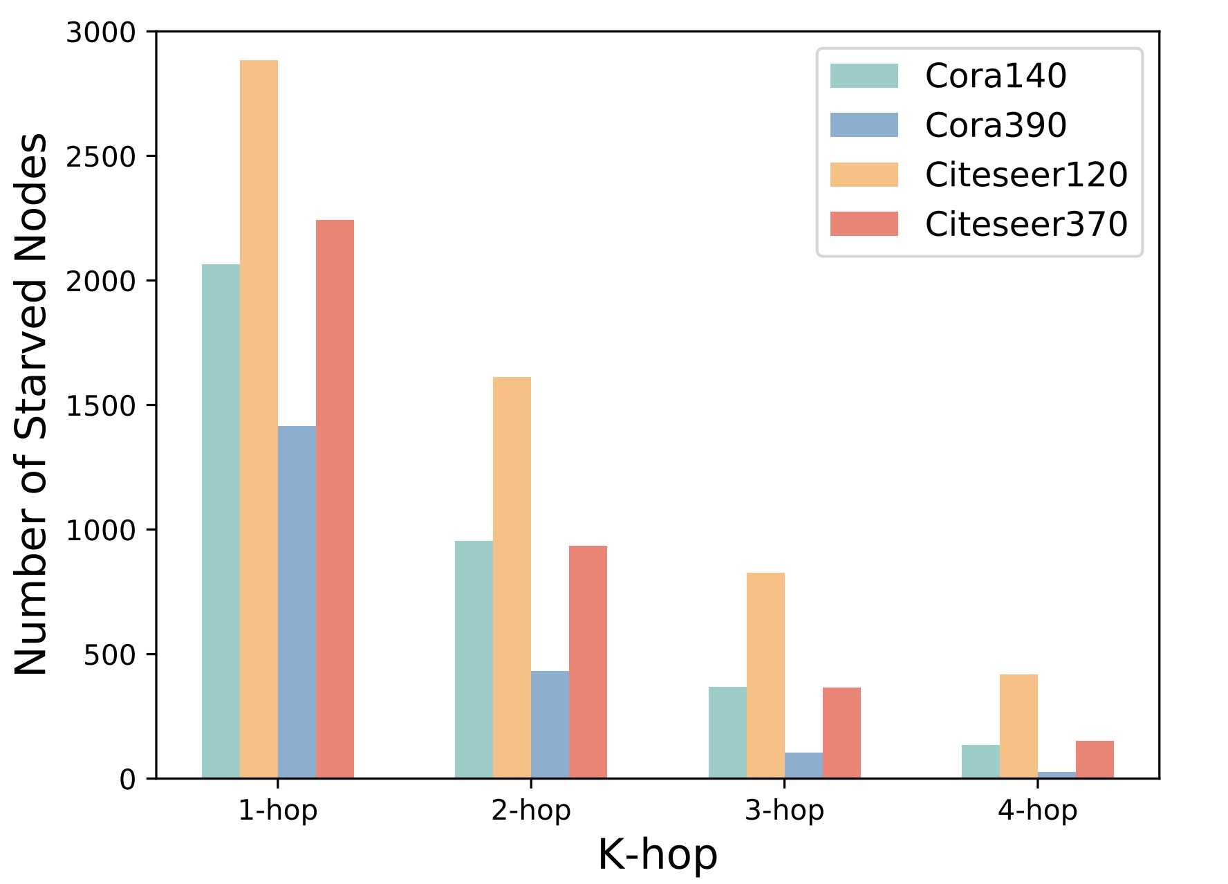
We observe that, there are many nodes suffer from the supervision starvation problem. The larger the labeling rate (i.e., the more labeled nodes), the smaller the number of starved nodes. This is natural because the more labeled nodes, the greater the probability that a node will connect to a labeled node. On the other hand, the number of k-hop starved nodes decreases as the value of k increases. Taking the Citeseer120 dataset as an example, increasing GNN to 4 layers (capturing 4-hop neighbors) reduces the number of starved nodes from near 3,000 to near 500. This can be explained by the fact that as k increases, the nodes have more neighbors (from 1- to k-hop), and the possibility of having at least one labeled neighbor increases.

How to Identify Starved Nodes

After define the k-hop starved nodes, we show how to identify such nodes based on a given initial adjacency matrix. The following theorem gives a solution.

[Theorem 1] Given a sparse adjacency matrix $\mathbf{A} \in \mathbb{R}^{n\times n}$ with self-connections generated on graph $\mathcal{G}(\mathcal{V}, \mathbf{X})$ by a latent graph inference model with a $k$-layer graph neural network $\mathtt{GNN}_k(\mathbf{X}; \mathbf{\Theta)}$, the node $V_i$ is a $k$-hop starved node, if $\exists j \in \{1, \ldots, n\}$, such that $[\mathbb{1}_{\mathbb{R}^+}(\mathbf{A})]^k_{ij}=1$, and for $\forall j \in \{j\ |\ [\mathbb{1}_{\mathbb{R}^+}(\mathbf{A})]_{ij}=1 \cup [\mathbb{1}_{\mathbb{R}^+}(\mathbf{A})]^2_{ij}=1 \cup \ldots \cup [\mathbb{1}_{\mathbb{R}^+}(\mathbf{A})]^k_{ij}=1 \}$, $V_j$ is unlabeled.

To provide a clearer understanding, we present an example to illustrate the process of identifying $k$-hop starved nodes based on the given adjacency matrix. The following figure depicts a graph consisting of $6$ nodes, with $2$ labeled and $4$ unlabeled. The corresponding adjacency matrix is shown in the right, where all edge weights are set to $1$ for simplicity. To identify the $k$-hop starved nodes, we need to determine the $k$-hop neighbors for each node. The steps below demonstrate the identification process of $k$-hop neighbors based on the given adjacency matrix, where the $k$-hop neighbors for each node are listed at the end of each row of the corresponding matrices:

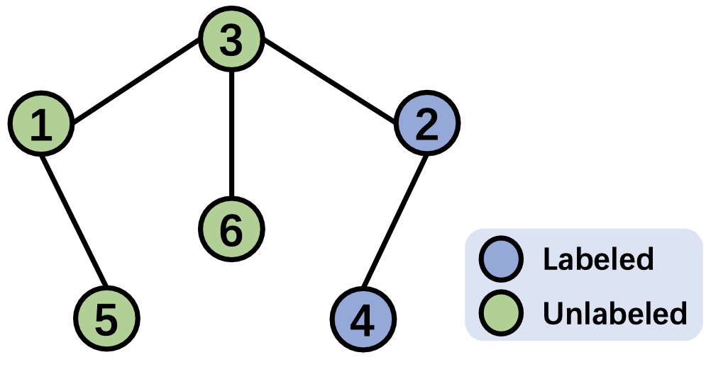
\begin{equation} \qquad\quad \end{equation}

\begin{equation} \mathbf{A}: \begin{array}{lll} & \begin{array}{llllll}\ \ 1 & 2 & 3 & 4 & 5 & 6 \end{array} & \\ \begin{array}{l} 1 \\ 2 \\ 3 \\ 4 \\ 5 \\ 6 \end{array}& \left[\begin{array}{llllll} 1 & 0 & 1 & 0 & 1 & 0 \\ 0 & 1 & 1 & 1 & 0 & 0 \\ 1 & 1 & 1 & 0 & 0 & 1 \\ 0 & 1 & 0 & 1 & 0 & 0 \\ 1 & 0 & 0 & 0 & 1 & 0 \\ 0 & 0 & 1 & 0 & 0 & 1 \\ \end{array}\right] \begin{array}{l} \end{array} \end{array} \nonumber \end{equation}

\begin{equation} \text{Identifying $1$-hop neighbors based on }\mathbf{A}: \begin{array}{lll} & \begin{array}{llllll}\ \ 1 & 2 & 3 & 4 & 5 & 6 \end{array} & \\ \begin{array}{l} 1 \\ 2 \\ 3 \\ 4 \\ 5 \\ 6 \end{array}& \left[\begin{array}{llllll} 1 & 0 & 1 & 0 & 1 & 0 \\ 0 & 1 & 1 & 1 & 0 & 0 \\ 1 & 1 & 1 & 0 & 0 & 1 \\ 0 & 1 & 0 & 1 & 0 & 0 \\ 1 & 0 & 0 & 0 & 1 & 0 \\ 0 & 0 & 1 & 0 & 0 & 1 \\ \end{array}\right] \begin{array}{l} (V_3, V_5) \\ (V_3, {V_4}) \\ (V_1, {V_2}, V_6) \\ ({V_2}) \\ (V_1) \\ (V_3) \end{array} \end{array} \nonumber \end{equation}

Since nodes $V_2$ and $V_4$ are labeled, we identify the $1$-hop starved nodes as $\{V_1, V_5, V_6\}$ (we want to clarify that self-connections are not considered when defining k-hop neighbors.).

\begin{equation} \text{Identifying $2$-hop neighbors based on }\mathbf{A}^2: \begin{array}{lll} & \begin{array}{llllll}\ \ 1 & 2 & 3 & 4 & 5 & 6 \end{array} & \\ \begin{array}{l} 1 \\ 2 \\ 3 \\ 4 \\ 5 \\ 6 \end{array}& \left[\begin{array}{llllll} 3 & 1 & 2 & 0 & 2 & 1 \\ 1 & 3 & 2 & 2 & 0 & 1 \\ 2 & 2 & 4 & 1 & 1 & 2 \\ 0 & 2 & 1 & 2 & 0 & 0 \\ 2 & 0 & 1 & 0 & 2 & 0 \\ 1 & 1 & 2 & 0 & 0 & 2 \\ \end{array}\right] \begin{array}{l} ({V_2}, V_6) \\ (V_1, V_6) \\ ({V_4}, V_5) \\ (V_3) \\ (V_3) \\ (V_1, {V_2}) \end{array} \end{array} \nonumber \end{equation}

Now, we can identify $2$-hop starved nodes from the set $\{V_1, V_5, V_6\}$ as $\{V_5\}$.

\begin{equation} \text{Identifying $3$-hop neighbors based on }\mathbf{A}^{3}: \begin{array}{lll} & \begin{array}{llllll}\ \ 1 & 2 & 3 & \ \ 4 & 5 & 6 \end{array} & \\ \begin{array}{l} 1 \\ 2 \\ 3 \\ 4 \\ 5 \\ 6 \end{array}& \left[\begin{array}{llllll} 7 & 3 & 7 & 1 & 5 & 3 \\ 3 & 7 & 7 & 5 & 1 & 3 \\ 7 & 7 & 10 & 3 & 3 & 6 \\ 1 & 5 & 3 & 4 & 0 & 1 \\ 5 & 1 & 3 & 0 & 4 & 1 \\ 3 & 3 & 6 & 1 & 1 & 4 \\ \end{array}\right] \begin{array}{l} (V_4) \\ (V_5) \\ (\varnothing) \\ (V_1,V_6) \\ (V_2,V_6) \\ (V_4,V_5) \end{array} \end{array} \nonumber \end{equation}

We observe that there are no $3$-hop starved nodes.

\begin{equation} \text{Identifying $4$-hop neighbors based on }\mathbf{A}^4: \begin{array}{lll} & \begin{array}{llllll}\ \ \ 1 & \ \ 2 & \ \ 3 & \ 4 & \ \ \ 5 &\ \ 6 \end{array} & \\ \begin{array}{l} 1 \\ 2 \\ 3 \\ 4 \\ 5 \\ 6 \end{array}& \left[\begin{array}{llllll} 19 & 11 & 20 & 4 & 12 & 10 \\ 11 & 19 & 20 & 12 & 4 & 10 \\ 20 & 20 & 30 & 10 & 10 & 16 \\ 4 & 12 & 10 & 9 & 1 & 4 \\ 12 & 4 & 10 & 1 & 9 & 4 \\ 10 & 10 & 16 & 4 & 4 & 10 \\ \end{array}\right] \begin{array}{l} (\varnothing) \\ (\varnothing) \\ (\varnothing) \\ (V_5) \\ (V_4) \\ (\varnothing) \end{array} \end{array} \nonumber \end{equation}

We observe that there are no $4$-hop starved nodes.

Note that, a node identified as $k$-hop starved node is also considered as a $(k-1)$-hop starved node, as exemplified by node $V_5$. Consequently, if there are no $k$-hop starved nodes present, it follows that there are no $(k+1)$-hop starved nodes.

CUR Decomposition Makes A Better Solution

Although the above strategy is effective to identify starved nodes, it is computationally complex. Even with a small value of $k$, the computational cost of identifying $k$-hop starved nodes based on such strategy is prohibitively expensive. For example, when identifying $2$-hop starved nodes, the time complexity of computing $\mathbf{A}^2$ alone reaches $\mathcal{O}(n^3)$. To solve this problem, we provide a more efficient alternative approach inspired by matrix CUR decomposition:

[Definition 3] (CUR Decomposition) Given $\mathbf{Q} \in \mathbb{R}^{n\times m}$ of rank $\rho=\mathtt{rank}(\mathbf{Q})$, rank parameter $k < \rho$, and accuracy parameter $0 < \varepsilon < 1$, construct column matrix $\mathbf{C} \in \mathbb{R}^{n\times c}$ with $c$ columns from $\mathbf{Q}$, row matrix $\mathbf{R} \in \mathbb{R}^{r\times m}$ with $r$ rows from $\mathbf{Q}$, and intersection matrix $\mathbf{U} \in \mathbb{R}^{c\times r}$ with $c$, $r$, and $\mathtt{rank}(\mathbf{U})$ being as small as possible, in oder to reconstruct $\mathbf{Q}$ within relative-error: \begin{equation} ||\mathbf{Q}-\mathbf{CUR}||_F^2 \leq (1+\varepsilon)||\mathbf{Q}-\mathbf{Q}_k||_F^2. \end{equation} Here, $\mathbf{Q}_k = \mathbf{U}_k \mathbf{\Sigma}_k \mathbf{V}_k^T \in \mathbb{R}^{n\times m}$ is the best rank $k$ matrix obtained via the singular value decomposition (SVD) of $\mathbf{Q}$.

With the definition of CUR decomposition, we can find a more efficient solution to identify the starved nodes. The following theorem demonstrates how we can accomplish this goal.

[Theorm 2] Given a sparse adjacency matrix $\mathbf{A} \in \mathbb{R}^{n\times n}$ with self-connections generated on graph $\mathcal{G}(\mathcal{V}, \mathbf{X})$, construct $\mathbf{C} = \mathbf{A}[:, col\_mask] \in \mathbb{R}^{n\times c}$, where $col\_mask \in \{0, 1\}^{n}$ contains only $c$ positive values corresponding to $c$ labeled nodes, and $\mathbf{R} = \mathbf{A}[row\_mask, :] \in \mathbb{R}^{r\times n}$ with $row\_mask = \mathbb{1}_{\mathbb{R}^-}(\mathbf{C}\mathbb{1}_c) \in \{0, 1\}^{n}$. Then, (a) ${\mathbf{U}} = \mathbf{A}[row\_mask, col\_mask] = \mathbf{0} \in \mathbb{R}^{r\times c}$, where $\mathbf{0}$ is a zero matrix, (b) the set of $1$-hop starved nodes $\texttt{Set}_1(r) = \{V_i | i \in {\texttt{RM}_+} \} $, where $\texttt{RM}_+ \in \mathbb{N}^r$ indicates the set of indexes of positive elements from $row\_mask$, and (c) for each $i \in \texttt{RM}_+$, $V_i$ is a $2$-hop starved node if, for $\forall j$ satisfying $[\mathbb{1}_{\mathbb{R}^+}(\mathbf{R})]_{ij}=1$, $j \in \texttt{RM}_+$.

The above theorem provides a more efficient alternative for identifying $k$-hop starved nodes for $k\in \{1, 2\}$. In fact, the column matrix $\mathbf{C}$ models the relationships between all nodes and $c$ labeled nodes, the row matrix $\mathbf{R}$ models the affinities between $r$ $1$-hop starved nodes and the whole nodes, and the intersection matrix ${\mathbf{U}}$ models the strength of connections between $r$ $1$-hop starved nodes and $c$ labeled nodes. This theorem states that ${\mathbf{U}}=\mathbf{0}$, indicting that there are no connections between the starved nodes and the labeled ones. For better illustration, we show the $\mathbf{C}$, $\mathbf{U}$, and $\mathbf{R}$ matrices of the above adjacency matrix as follows:

\begin{equation} \mathbf{C} : \begin{array}{lll} & \begin{array}{ll}\ \ \ 2 & 4 \end{array} & \\ \begin{array}{l} 1 \\ 2 \\ 3 \\ 4 \\ 5 \\ 6 \end{array}& \left[\begin{array}{llll} 0 & 0 \\ 1 & 1 \\ 1 & 0 \\ 1 & 1 \\ 0 & 0 \\ 0 & 0 \\ \end{array}\right] \end{array}; \quad\qquad \mathbf{R} : \begin{array}{lll} & \begin{array}{llllll} \ \ 1 & 2 & 3 & 4 & 5 & 6 \end{array} & \\ \begin{array}{l} 1 \\ 5 \\ 6 \end{array}& \left[\begin{array}{llllll} 1 & 0 & 1 & 0 & 1 & 0 \\ 1 & 0 & 0 & 0 & 1 & 0 \\ 0 & 0 & 1 & 0 & 0 & 1 \\ \end{array}\right] \end{array}; \quad\qquad \mathbf{U} : \begin{array}{lll} & \begin{array}{ll} \ \ 2 & 4 \end{array} & \\ \begin{array}{l} 1 \\ 5 \\ 6 \end{array}& \left[\begin{array}{ll} 0 & 0 \\ 0 & 0 \\ 0 & 0 \\ \end{array}\right] \end{array} \nonumber \end{equation}

Based on the $\mathbf{C}, \mathbf{U}, \mathbf{R}$ matrices, we can determine that $row\_mask = [1, 0, 0, 0, 1, 1]^{\top}$, $\texttt{RM}_+=\{1, 5, 6\}$, the $1$-hop starved nodes are $V_1, V_5, V_6$, and the $2$-hop starved node is $V_5$.

How to Eliminate Starved Nodes

After identification, we can reduce the starved nodes by rebuilding the corrupted affinities. Specifically, we reconstrcut the intersection matrix ${\mathbf{U}}$ to ensure that the reconstructed $\widetilde{\mathbf{U}} \neq \mathbf{0}$. Consequently, the rebuilt adjacency matrix can be rewritten as: \begin{equation} \widetilde{\mathbf{A}}^{} = \mathbf{A}_{} + \alpha \mathbf{B} = \mathbf{A}_{} + \alpha \Gamma\left(\widetilde{\mathbf{U}}, n\right), \label{equation5} \end{equation} where function $\Gamma(\widetilde{\mathbf{U}}, n)$ extends the matrix $\widetilde{\mathbf{U}}\in \mathbb{R}^{r\times c}$ to an $n \times n$ matrix by padding $n-r$ rows of zeros and $n-c$ columns of zeros in the corresponding positions. In fact, with the reconstructed $\widetilde{\mathbf{U}}$, we can also set $\widetilde{\mathbf{Q}}=\mathbf{C\widetilde{U}R}$ as the regularization $\mathbf{B}$. It is, of course, sensible and feasible. However, a potential drawback is that the reconstruction of $\widetilde{\mathbf{Q}}$ requires matrix multiplications of three matrices, which is time-consuming. Unexpectedly, we find that only constructing matrix $\widetilde{\mathbf{U}}$ is enough to solve the SS problem since it models the relationships between $1$-hop starved nodes and labeled ones.

The question now turns to how to reconstruct the intersection matrix $\widetilde{\mathbf{U}}$. For simplicity, we directly adopt the same strategy used in constructing $\mathbf{A}_{}$. Specifically, for each row $i$ of $\widetilde{\mathbf{U}}$, we establish a connection between $V_i$ and $V_j$ for $\forall j \in {\texttt{CM}_+}$, where ${\texttt{CM}_+} \in \mathbb{N}^c$ represents the set of indexes of positive elements from $col\_mask$. We then assign weights to these connections based on their distance. Note that, if we ensure each row of $\widetilde{\mathbf{U}}$ has at least one weight greater than 0, there will be no $\kappa$-hop starved nodes for $\forall \kappa > 1$. This means that we do not need to feed the $k$-hop starved nodes satiated, simply feeding $\kappa$-hop ones for $\forall \kappa < k$ makes $k$-hop starved nodes cease to exist.

Experiments

BibTeX

@inproceedigs{Jianglin2023LGI,
title={Latent Graph Inference with Limited Supervision},
author={Lu, Jianglin and Xu, Yi and Wang, Huan and Bai, Yue and Fu, Yun},
booktitle={Advances in Neural Information Processing Systems},
year={2023}
}

This website is borrowed from nerfies.